When we think about statistics, one curve tends to appear again and again — the Normal Distribution. If you’ve ever heard of the “bell curve,” you’ve already encountered it. This simple but powerful concept sits at the heart of probability, data analysis, machine learning, and even everyday decision-making.
What is the Normal Distribution?
The normal distribution is a continuous probability distribution that is symmetrical around its mean. In plain terms, most of the data points cluster around the center, and fewer observations occur as we move further away in either direction.
It’s often called the Gaussian distribution or the bell curve because of its characteristic shape.
If we take any dataset and plot a histogram, a bell-like shape hints at normally distributed data.
Key Features of the Normal Distribution
- Symmetry: The left and right sides of the curve are mirror images.
- Bell Shape: Most data cluster around the center with tails that taper off.
- Equal Mean, Median, and Mode: All three lie at the center of the curve.
- Spread Defined by σ (Standard Deviation):
- A smaller σ gives a narrow, steep curve.
- A larger σ produces a wider, flatter curve.
- Total Area = 1: The curve represents 100% probability.
In formula form, the normal distribution looks like this:
f(x|\mu,\sigma^2) = \frac{1}{\sqrt{2\pi\sigma^2}} e^{ -\frac{(x-\mu)^2}{2\sigma^2} }
Here:
- μ = mean (center of the curve)
- σ = standard deviation (spread of data)
- e = Euler’s number (~2.718)
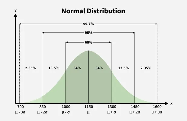
The 68-95-99.7 Rule
One of the most famous properties of the bell curve is how much data falls within standard deviations of the mean:
- 68% within 1 standard deviation (μ ± 1σ)
- 95% within 2 standard deviations (μ ± 2σ)
- 99.7% within 3 standard deviations (μ ± 3σ)
This rule makes the normal distribution extremely useful in real-world problem solving.
Real-World Applications
Normal distributions show up everywhere:
- Education: Standardized test scores (SAT, GRE, IQ).
- Healthcare: Blood pressure, cholesterol levels, patient response times.
- Business & Finance: Stock returns, risk management, financial modeling.
- Manufacturing: Quality control, defect detection, Six Sigma.
Whenever we deal with naturally occurring variation, chances are a normal curve is nearby.
Standard Normal Distribution
Sometimes, it’s easier to work with a “normalized” version of the bell curve where:
- Mean = 0
- Standard Deviation = 1
This is called the Standard Normal Distribution.
Enter the Z-Score
To convert any normally distributed data into the standard normal form, we use a Z-score:
z = \frac{x – \mu}{\sigma}
This process is called standardization. It tells us how many standard deviations away a data point lies from the mean.
Applications of Z-Score
- Standardizing Data: Brings different datasets to a common scale.
- Outlier Detection: Points with Z > 2 or 3 are often treated as unusual.
- Probabilities & Percentiles:
- A Z of 1.96 corresponds to the 97.5th percentile.
- This is the basis for the 95% confidence interval.
- Hypothesis Testing & Confidence Intervals in statistics.
- Feature Scaling in machine learning.
- Comparisons Across Populations — e.g., comparing two exam scores from different tests.
- Quality Control & Six Sigma.
Wrapping Up
The Normal Distribution is more than just a neat curve in a statistics textbook. It’s the backbone of probability theory and data analysis, powering applications from medical research to finance to AI.
Once you understand the bell curve and the Z-score, you unlock a powerful way to interpret uncertainty, detect anomalies, and make predictions.
So, the next time you see a dataset forming that familiar bell shape, you’ll know you’re looking at one of the most important patterns in all of statistics.